





Introduction
AutoML is a relatively new and upcoming subset of machine learning. The main approach in AutoML is to limit the involvement of data scientists and let the tool handle all time-consuming processes in machine learning like data preprocessing, best algorithm selection, hyperparameter tuning, etc., thus saving time for setting up these ML models and speeding up their deployment. There are several AutoML tools available in the market these days.
In one of my previous blogathon articles, I had shared a comprehensive guide to AutoML with an easy AutoGluon example. This guide included a list of several AutoML tools currently available in the market. These AutoML tools can undoubtedly save a good amount of time, especially for a large and complex dataset. We will explore one such tool called ‘Auto-Sklearn’ in this article.
What is Auto-Sklearn?
Anyone familiar with machine learning knows about scikit-learn, the famous python package consisting of different classification and regression algorithms and is used for building machine learning models.
Auto-Sklearn is a Python-based open-source toolkit for doing AutoML. It employs the well-known Scikit-Learn machine learning package for data processing and machine learning algorithms. It also includes a Bayesian Optimization search technique to find the best model pipeline for the given dataset quickly. In this article, we’ll look at how to utilize Auto-Sklearn for classification and regression tasks.
Let us install the Auto-Sklearn package first.
pip install auto-sklearn
(If you are using google colab, ensure your SciPy version is the latest; else upgrade it using pip command and restart the runtime)
pip install --upgrade scipy
Now that we have installed the AutoML tool, we will import the basic packages for preprocessing the dataset and visualization.
import pandas as pd
import numpy as np
import matplotlib.pyplot as plt
import seaborn as sns
from sklearn.model_selection import train_test_split
Classification Task
We will use the heart disease prediction dataset available on the UCI repository. For convenience, let us use the .csv version of this data from Kaggle. You can also use any classification dataset of your choice or import a toy dataset available from the sklearn library.
Dataset details: This dataset contains 303 samples and 14 attributes (the original dataset has 76 features while the .csv version has the 14 subsets of the original dataset).
Importing the dataset and printing first few rows
df=pd.read_csv('/content/heart.csv')
df.head()
Let us check the target variable ‘target’ in the dataset
df['target'].value_counts()

There are only two classes (0= healthy, 1= heart disease), so this is a binary classification problem. Also, This indicates that this is an imbalanced dataset. Due to this, the accuracy score of this model will be less reliable. However, we will first test the imbalanced dataset by directly feeding it to the autosklearn classifier. Later we will adjust the number of samples for these two classes and test the accuracy to see how the classifier performs.
#creating X and y
X=df.drop(['target'],axis=1)
y=df['target']
#split into train and test sets
X_train, X_test, y_train, y_test= train_test_split(X,y, test_size=0.2, random_state=42)
X_train.shape, X_test.shape,y_train.shape, y_test.shape

Next, we will import the classification models from autosklearn using the following command.
import autosklearn.classification
Then we will create an instance of the AutoSklearnClassifier for the classification task.
automl = autosklearn.classification.AutoSklearnClassifier( time_left_for_this_task=5*60,per_run_time_limit=30,tmp_folder='/temp/autosklearn_classification_example_tmp')
Here, we are setting the max time for this task using the ‘time_left_for_this_task’ argument and assigning 5*60 sec or 5 mins to it. If nothing is specified for this argument, the process will run for an hour, i.e., 60mins. Then, we will also set the time allocated as 30sec to each model evaluation using the “per_run_time_limit” argument.
In this command, there are other arguments like n_jobs (number of parallel jobs), ensemble_size, initial_configurations_via_metalearning, which can be used to fine-tune the classifier. By default, the above search command creates an ensemble of top-performing models. In order to avoid overfitting, we can disable it by changing the setting “ensemble_size” = 1 and “initial_configurations_via_metalearning” = 0. We have excluded these while setting up the classifier to keep the tutorial simple.
We will also provide a temporary path for the log to be saved, and we can use it to print the run details later.
Now, we will fit the classifier.
automl.fit(X_train, y_train)
The sprint_statistics() function summarizes the above search and the performance of the selected best model.
pprint(automl.sprint_statistics())

Alternatively, we can also print a leaderboard for all the models considered by the search, organized by their ranks using the following command.
print(automl.leaderboard())
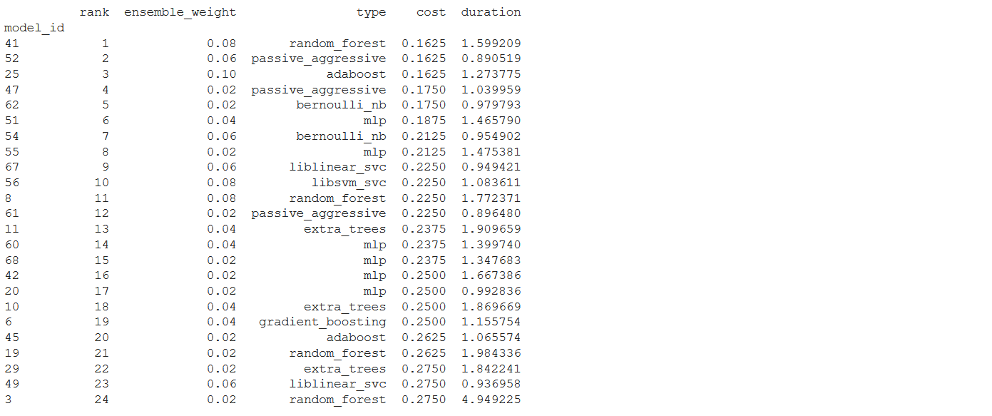
The top two models selected by the classifier were Random forest and Passive_aggressive respectively.
Additionally, we can print the information about the considered models using the following command:
pprint(automl.show_models())
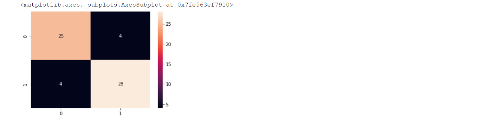
Lastly, we can also print the final score of the ensemble and the confusion matrix using the following lines of code.
# Score of the final ensemble
from sklearn.metrics import accuracy_score
m1_acc_score= accuracy_score(y_test, y_pred)
m1_acc_score
from sklearn.metrics import confusion_matrix, accuracy_score
y_pred= automl.predict(X_test)
conf_matrix= confusion_matrix(y_pred, y_test)
sns.heatmap(conf_matrix, annot=True)
We can use the following command to separate healthy and unhealthy samples in the dataset.
from sklearn.utils import resample
healthy= df[df["target"]==0]
unhealthy=df[df["target"]==1]
As the number of unhealthy samples is more, we will use the resampling technique (oversampling) and increase the samples of healthy individuals in the dataset. To adjust the skew, we can use the following commands –
up_sampled=resample(healthy, replace=True, n_samples=len(unhealthy), random_state=42)
up_sampled=pd.concat([unhealthy, up_sampled])
#check updated class counts
up_sampled['target'].value_counts()
We can also use techniques like SMOTE, Ensemble learning (bagging, boosting), NearMiss Algorithm to address the imbalance in the dataset. Additionally, we can use metrics such as F1-score, precision, and recall to evaluate the model’s performance.
Now that we have adjusted the skew, we will create X and y sets for classification again. Let us name them X1 and y1 to avoid confusion.
X1=up_sampled.drop(['target'],axis=1)
y1=up_sampled['target']
We need to repeat all the steps from setting up the classifier to printing a confusion matrix for this new X1 and y1. Complete code for this task is available on my GitHub repository.
Finally, we can compare the two accuracies for skewed data and adjusted data using –
model_eval = pd.DataFrame({'Model': ['skewed','adjusted'], 'Accuracy': [m1_acc_score,m2_acc_score]})
model_eval = model_eval.set_index('Model').sort_values(by='Accuracy',ascending=False)
fig = plt.figure(figsize=(12, 4))
gs = fig.add_gridspec(1, 2)
gs.update(wspace=0.8, hspace=0.8)
ax0 = fig.add_subplot(gs[0, 0])
sns.heatmap(model_eval,cmap="PiYG",annot=True,fmt=".1%", linewidths=4,cbar=False,ax=ax0)
plt.show()
From the above chart, the model accuracy has slightly reduced after over-sampling, we can see that the model is now better optimized. Although we have used quite a few additional commands for preprocessing the data and evaluating the results, running an AutoSklearn classifier requires only one single line of code. Even with skewed data, the accuracy achieved by the model is really good.
Regression Task
Now we will use the Regression models from AutoSklearn in this section.
For this task, let us use the simple ‘flights’ dataset from the seaborn datasets library. We will load the dataset with the following command.
#loading the dataset
df = sns.load_dataset('flights')
df.head()
Dataset details: This dataset contains 144 rows and 3 columns, namely year, month, and the number of passengers.
The task here is to predict the number of passengers using the other two features.
X=df.drop(["passengers"],axis=1)
y=df["passengers"]
X.shape, y.shape

X_train, X_test, y_train, y_test = train_test_split(X, y, test_size=0.2, random_state=42)
X_train.shape, X_test.shape,y_train.shape, y_test.shape

We now use autosklearnregressor for this regression task.
import autosklearn.regression
automl = autosklearn.regression.AutoSklearnRegressor(
time_left_for_this_task=5*60,per_run_time_limit=30,tmp_folder='/temp/autosklearn_regression_example_tmp')
automl.fit(X_train, y_train)
from sklearn.metrics import mean_absolute_error
from autosklearn.metrics import mean_absolute_error as auto_mean_absolute_error
Now, let us print the statistics of the model.
# summarize
print(automl.sprint_statistics())

From the above-printed summary, we understand that the regressor ran a total of 59 models, and the calculated performance of the final regression model was R2 of 0.985, which is quite good.
Since the regressor has optimized the R2 metric by default, let us print the mean absolute error to evaluate the performance of the model better.
# evaluate the best model
y_pred = automl.predict(X_test)
mae = mean_absolute_error(y_test, y_pred)
print("MAE: %.3f" % mae)
The mean absolute error is acceptable looking at the R2 value achieved by the model and the size of the example dataset used for this task.
We can also plot the predicted values against the actual values using matplotlib as shown below.
plt.figure(figsize=(8,6))
plt.scatter(y_test, y_pred, c='blue')
p1 = max(max(y_pred), max(y_test))
p2 = min(min(y_pred), min(y_test))
plt.plot([p1, p2], [p1, p2], 'r-')
plt.xlabel('Actual', fontsize=10)
plt.ylabel('Predicted', fontsize=10)
plt.legend(['Actual', 'Predicted'])
plt.axis('equal')
plt.show()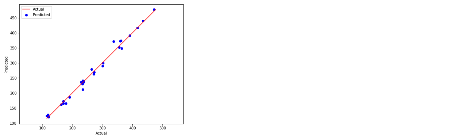
Overall, we can say that the MAE value is small, and the model achieved a high validation score is 0.985, indicating that the model performance is good.
Saving the trained models.
The above-trained models for classification and regression can be saved using python packages Pickle and JobLib. These saved models can then be used to make predictions directly on new data. We can save the models as:
1. Using
Pickle
import pickle
# save the model
filename = 'final_model.sav'
pickle.dump(model, open(filename, 'wb'))
Here ‘wb’ argument means that we are writing the file to the disk in binary mode. Further, we can load this saved model as :
#load the model
loaded_model = pickle.load(open(filename, 'rb'))
result = loaded_model.score(X_test, Y_test)
print(result)
Here ‘rb’ command indicates we are reading the file in binary mode.
2. Using
JobLib
Similarly, we can save the trained models in JobLib using the following command.
import joblib
# save the model
filename = 'final_model.sav'
joblib.dump(model, filename)
We can also reload these saved models later for predictions on new data.
# load the model from disk
load_model = joblib.load(filename)
result = load_model.score(X_test, Y_test)
print(result)
Conclusion
In this article, we saw the application of the Auto-Sklearn for both classification and regression models. For both tasks, we did not require to specify a particular algorithm. Instead, the tool itself iterated through several inbuilt algorithms and achieved good results (higher accuracy in the classification model and lower mean absolute error in the regression model). Thus, AutoSklearn can be a valuable tool to build better machine learning models with a few lines of code. The complete tutorial for this article is available on my GitHub repository.


