The field of graph machine learning has grown rapidly in recent times, and most models in this field are implemented in Python. This article will introduce graphs as a concept and some rudimentary ways of dealing with them using Python. After that we will create a graph convolutional network and have it perform node classification on a real-world relationship network with the help of PyTorch. The whole workflow described here is available as a Colab Notebook.

What is a graph?

A graph, in its most general form, is simply a collection of nodes along with a set of edges between the nodes. Formally, a graph G can be written as G = (V, E)where V represents the nodes and E the corresponding set of edges. There are two main types of graphs, directed and undirected. The edges of directed graph point from their origin u node towards the target node v, whereas edges in undirected graphs are without direction such that (u, v) ∈ E ⇔ (v, u) ∈ E. Graphs can be represented through an adjacency matrix A.This matrix can be created by having every node index a particular row and column. The presence of edges can then be represented as entries in the adjacency matrix, meaning that A[u, v] = 1 if (u, v) ∈ E and A[u, v] = 0, otherwise. The adjacency matrix will be symmetric if the graph is made up of only undirected edges, but if the graph is directed that won’t necessarily be the case.

To operate on graphs in Python, we will use the highly popular networkx library [1]. We start by creating an empty directed graph H:

import networkx as nxH = nx.DiGraph()

We will then add 4 nodes to the graph. Each node has 2 features attached to it, color and size. It is common for graphs in machine learning problems to have nodes with features, such as the name or age of a person in a social network, which can then be used by the model to infer complex relations and make predictions. Networkx comes with a built in utility function for filling a graph with nodes as a list, in addition to their features:

H.add_nodes_from([
  (0, {"color": "gray", "size": 450}),
  (1, {"color": "yellow", "size": 700}),
  (2, {"color": "red", "size": 250}),
  (3, {"color": "pink", "size": 500})
])for node in H.nodes(data=True):
  print(node)> (0, {'color': 'gray', 'size': 450})
> (1, {'color': 'yellow', 'size': 700})
> (2, {'color': 'red', 'size': 250})
> (3, {'color': 'pink', 'size': 500})

An edge in the graph is defined as a tuple containing the origin and target node, so for example the edge (2, 3) connects node 2 to node 3. Since we have a directed graph, there can also be an edge (3, 2) which points in the opposite direction. Multiple edges can be added to the graph as part of a list in a similar manner as nodes can:

H.add_edges_from([
  (0, 1),
  (1, 2),
  (2, 0),
  (2, 3),
  (3, 2)
])print(H.edges())> [(0, 1), (1, 2), (2, 0), (2, 3), (3, 2)]

Now that we have created a graph, let’s define a function to display some information about it. We validate that the graph is indeed directed and that it has the correct number of nodes as well as edges.

def print_graph_info(graph):
  print("Directed graph:", graph.is_directed())
  print("Number of nodes:", graph.number_of_nodes())
  print("Number of edges:", graph.number_of_edges())print_graph_info(H)> Directed graph: True
> Number of nodes: 4
> Number of edges: 5

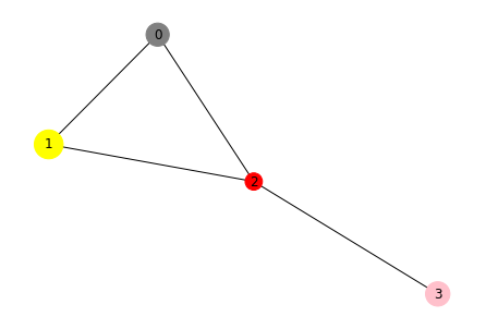
It can also be very helpful to plot a graph that you are working with. This can be achieved using nx.draw. We use the nodes’ features to color each node and give each of them their own size in the plot. Since node attributes come as dictionaries, and the draw function only accepts lists we will have to convert them first. The resulting graph looks like it is supposed to with 4 nodes, 5 edges and the correct node features.

node_colors = nx.get_node_attributes(H, "color").values()
colors = list(node_colors)node_sizes = nx.get_node_attributes(H, "size").values()
sizes = list(node_sizes)nx.draw(H, with_labels=True, node_color=colors, node_size=sizes)

Let’s convert the directed graph H to an undirected graph G. After that we again print information about the graph and we can see that the conversion worked because the output indicates that it is not a directed graph anymore.

G = H.to_undirected()
print_graph_info(G)> Directed graph: False
> Number of nodes: 4
> Number of edges: 4

The number of edges has curiously decreased by one. If we take a closer look we can see that the edge (3, 2) has disappeared, which is reasonable since an undirected edge can be represented by only one tuple, in this case (2, 3).

print(G.edges())> [(0, 1), (0, 2), (1, 2), (2, 3)]

When we visualize the undirected graph, we can see that the directions of the edges have disappeared while everything else remain the same.

nx.draw(G, with_labels=True, node_color=colors, node_size=sizes)

The Karate Club Network

Now that we have a high-level understanding of how to deal with graphs in Python, we will take a look at a real world network that we can use to define a machine learning task on. Zachary’s Karate Club Network [2] is chosen for this purpose. It represents friendship relationships between members of a karate club studied by W. Zachary in the seventies. An edge in the graph connects two individuals if they socialize outside of the club.

The Karate Club dataset is available through PyTorch Geometric (PyG ) [3]. The PyG library contains all sorts of methods for deep learning on graphs and other irregular structures. We begin by inspecting some of the properties of the dataset. It seems to only contain one graph, which is expected since it depicts one club. Furthermore, each node in the dataset is assigned a 34 dimensional feature vector that uniquely represents every node. Every member of the club is part of one of 4 factions, or classes in machine learning terms.

from torch_geometric.datasets import KarateClubdataset = KarateClub()
print("Dataset:", dataset)
print("# Graphs:", len(dataset))
print("# Features:", dataset.num_features)
print("# Classes:", dataset.num_classes)> Dataset: KarateClub()
> # Graphs: 1
> # Features: 34
> # Classes: 4

We can further explore the only graph in the dataset. We see that the graph is undirected, and it has 34 nodes, each with 34 features as mentioned before. The edges are represented as tuples, and there are 156 of them. However, in PyG undirected edges are represented as two tuples, one for each direction, also known as bi-diretional, meaning that there are 78 unique edges in the Karate Club graph. PyG only include entries in A which are non-zero, which is why edges are represented like this. This type of representation is known as coordinate format, which is commonly used for sparse matrices. Each node has a label, y, that holds information about which class the corresponding node is part of. The data also contains a train_mask that has the indices of the nodes we know the ground truth labels for during training. There are 4 truth nodes, one for each faction, and the task at hand is then to infer the faction for the rest of the nodes.

data = dataset[0]print(data)
print("Training nodes:", data.train_mask.sum().item())
print("Is directed:", data.is_directed())> Data(x=[34, 34], edge_index=[2, 156], y=[34], train_mask=[34])
> Training nodes: 4
> Is directed: False

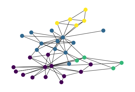
We convert the Karate Club Network to a Networkx graph, which allows us to use the nx.draw function to visualize it. The nodes are colored according to the class (or faction) they belong to.

from torch_geometric.utils import to_networkxG = to_networkx(data, to_undirected=True)
nx.draw(G, node_color=data.y, node_size=150)

Semi-supervised node classification

When training a model to perform node classification it can be referred to as semi-supervised machine learning, which is the general term used for models that combine labeled and unlabeled data during training. In the case of node classification we have access to all the nodes in the graph, even those belonging to the test set. The only information missing is the labels of the test nodes.

Graph Convolutional Networks (GCNs) will be used to classify nodes in the test set. To give a brief theoretical introduction, a layer in a graph neural network can be written as a non-linear function f:

that take as inputs the graph’s adjacency matrix A and (latent) node features H for some layer l. A simple layer-wise propagation rule for a graph neural network would look something like this:

where W is a weight matrix for the l-th neural network layer, and σ is a non-linear activation function. Multiplying the weights with the adjacency matrix means that all the feature vectors of all (1-hop) neighboring nodes are summed and aggregated for every node. However, the feature vector of the node itself is not included.

To address this, Kipf and Welling [4] add the identity matrix to the adjacency matrix and denote this new matrix  = A + I. Multiplication of the adjacency matrix will also change the scale of the feature vectors. To counteract this  is multiplied by its diagonal degree matrix symmetrically, yielding the final GCN propagation rule:

The GCN layer is already a part of what PyG, and it can be readily be imported as the GCNConv class. The same way layers can be stacked in normal neural networks, it is also possible to stack multiple GCN layers. Having a 3-layer GCN will result in three successive propagation steps, leading to every node being updated with information from 3 hops away. The first layer of the model must have as many input units as the number of features every node has. In line with the original GCN paper the latent dimensions are set to 4, apart from the last one, which is set to 2. This allows us to plot the learned latent embedding as a two dimensional scatter plot later on, to see if the model manages to learn embeddings that are similar for nodes belonging to the same class. The hyperbolic tangent activation function is used in-between GCN layers as a non-linearity. The output layer maps the 2 dimensional node embedding to 1 out of the 4 classes.

from torch.nn import Linear
from torch_geometric.nn import GCNConvclass GCN(torch.nn.Module):
  def __init__(self):
    super(GCN, self).__init__()
    torch.manual_seed(42)
    self.conv1 = GCNConv(dataset.num_features, 4)
    self.conv2 = GCNConv(4, 4)
    self.conv3 = GCNConv(4, 2)
    self.classifier = Linear(2, dataset.num_classes)  def forward(self, x, edge_index):
    h = self.conv1(x, edge_index)
    h = h.tanh()
    h = self.conv2(h, edge_index)
    h = h.tanh()
    h = self.conv3(h, edge_index)
    h = h.tanh()
    out = self.classifier(h)
    return out, hmodel = GCN()
print(model)> GCN(
>   (conv1): GCNConv(34, 4)
>   (conv2): GCNConv(4, 4)
>   (conv3): GCNConv(4, 2)
>   (classifier): Linear(in_features=2, out_features=4, bias=True)
> )

We use cross-entropy as loss functions since it is well suited for multi-class classification problems, and initialize Adam as a stochastic gradient optimizer. We create a standard PyTorch training loop, and let it run for 300 epochs. Note that while all nodes do indeed get updates to their node embeddings, the loss is only calculated for nodes in the training set. The loss is drastically decreased during training, meaning that the classification works well. The 2 dimensional embeddings from the last GCN layer are stored as a list so that we can animate the evolution of the embeddings during training, giving some insight into the latent space of the model.

criterion = torch.nn.CrossEntropyLoss()
optimizer = torch.optim.Adam(model.parameters(), lr=0.01)def train(data):
  optimizer.zero_grad()
  out, h = model(data.x, data.edge_index)
  loss = criterion(out[data.train_mask], data.y[data.train_mask])
  loss.backward()
  optimizer.step()
  return loss, hepochs = range(1, 301)
losses = []
embeddings = []for epoch in epochs:
  loss, h = train(data)
  losses.append(loss)
  embeddings.append(h)
  print(f"Epoch: {epoch}\tLoss: {loss:.4f}")> Epoch: 1    Loss: 1.399590
> Epoch: 2    Loss: 1.374863
> Epoch: 3    Loss: 1.354475
> ...
> Epoch: 299  Loss: 0.038314
> Epoch: 300  Loss: 0.038117

Matplotlib can be used to animate a scatter plot of the node embeddings where every dot is colored according to the faction they belong to. For every frame we display the epoch in addition to the training loss value for that epoch. Finally, the animation is converted to a GIF which is visible below.

import matplotlib.animation as animationdef animate(i):
  ax.clear()
  h = embeddings[i]
  h = h.detach().numpy()
  ax.scatter(h[:, 0], h[:, 1], c=data.y, s=100)
  ax.set_title(f'Epoch: {epochs[i]}, Loss: {losses[i].item():.4f}')
  ax.set_xlim([-1.1, 1.1])
  ax.set_ylim([-1.1, 1.1])fig = plt.figure(figsize=(6, 6))
ax = plt.axes()
anim = animation.FuncAnimation(fig, animate, frames=epochs)
plt.show()gif_writer = animation.PillowWriter(fps=20)
anim.save('embeddings.gif', writer=gif_writer)

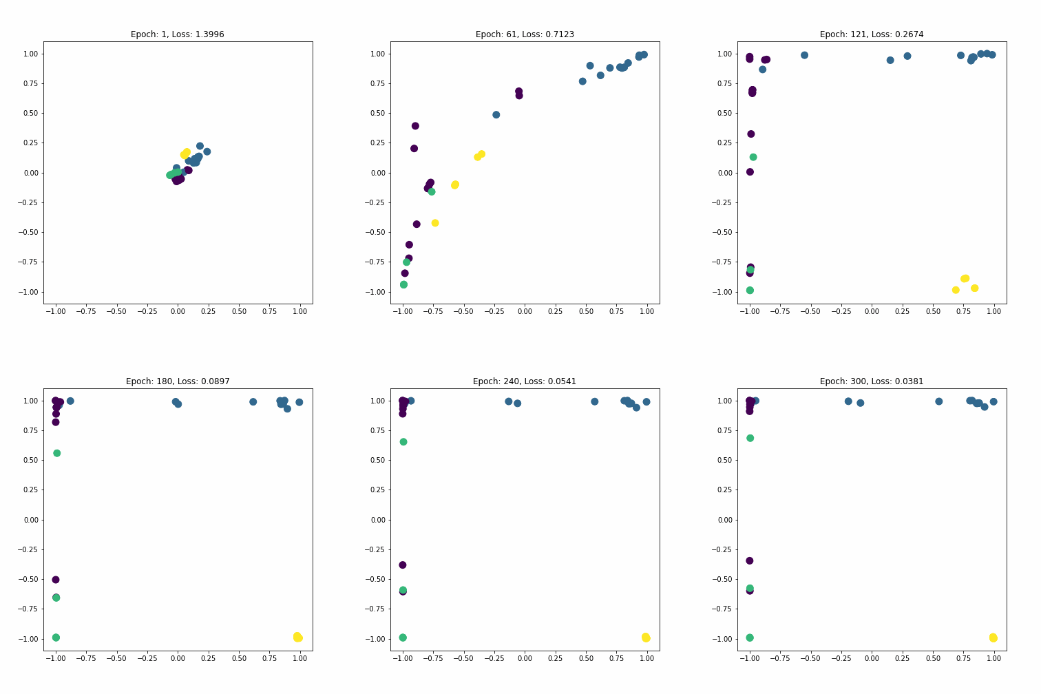
The GCN model manages to linearly separate almost all the nodes of different classes. This is impressive considering it was given only one labeled example per every faction as input.

Hopefully you found this introduction to graph neural networks interesting. GNNs are very versatile algorithms in that they can be applied to complex data and solve different types of problems. For example, by simply aggregating the node features using some permutation invariant pooling such as mean at the end of our neural network, it can do classification over the whole graph as opposed to over individual nodes!