Supervised machine learning is a technique that maps a series of inputs (X) to some known outputs (y) without being explicitly programmed. Training a machine learning model refers to the process where a machine learns a mapping between X and y. Once trained the model can be used to make predictions on new inputs where the output is unknown.
The training of a machine learning model is only one element of the end to end machine learning lifecycle. For a model to be truly useful this mapping needs to be stored and deployed for use. This is often referred to as putting the model into production. Additionally once a model is in production, the predictions and overall performance of the model need to be monitored to ensure that the quality of the predictions does not degrade over time.
To introduce the basic concepts in the end to end machine learning workflow I am going to use the python library, Pycaret. Pycaret is a low code machine learning library that seeks to simplify and speed up the overall machine learning workflow by providing a high-level programming interface and seeking to automate some of the repetitive tasks in machine learning.
The library is developing quickly and has more recently added functionality to encompass the entire end to end machine learning workflow. From model development to deployment and monitoring. In the following article, I will be using this package to give a simple introduction to the end to end machine learning lifecycle.
The data
In this tutorial, I am going to use one of Pycaret’s built-in datasets known as “employee”. This consists of a set of features about employees at an unspecified company and a target variable that denotes if that employee has left the company. This is a classic classification task in machine learning where the goal is to train a model that can predict if an employee is likely to leave.
The data can easily be imported through the Pycaret API. In the below code we read in the data and reserve a validation sample for later use in the workflow.https://towardsdatascience.com/media/a899a207623e8d3e70d169e4c4cf760d
The first few lines of the data look as follows:

Preprocessing
Pycaret has a set of modules that contain a suite of functions for a specific machine learning task. The dataset we are using contains a classification problem so we will be primarily using the classification module.
The first step is to import the setup function. This function is run prior to performing any other steps. It initialises the Pycaret environment and creates a transformation pipeline for preprocessing the data ready for modelling. When run Pycaret will infer the data types for all feature and target columns.https://towardsdatascience.com/media/458850891deec26ad914689011ae0ca4
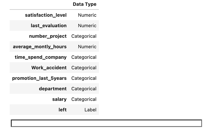
If we are happy that these data types are correct and are also happy to rely on Pycaret’s default preprocessing methods then we can simply hit enter and Pycaret will prepare the data for modelling, and print a report describing the steps that have been taken.
Below is just the first 15 lines of this 59 line report. The setup functions has a large number of optional parameters that can be used to create custom preprocessing. For example, the parameter categorical_features can be used to manually specify categorical columns where the data type has not been inferred correctly. A full list of available parameters can be found here.
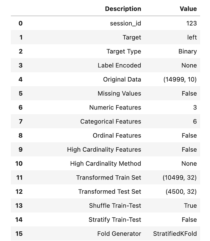
In a real-world machine learning project, it is likely that we would perform more in-depth exploratory analysis and custom preprocessing. However, for the purposes of this tutorial, we will continue with the default preprocessing.
Baseline model
Typically in machine learning workflows, it is sensible to train a simple model first to develop a baseline for performance before moving onto more complex algorithms.
At the time of writing, Pycaret supports 18 different algorithms for classification. The full list can be found here. For the baseline model, we will use logistic regression and we use the function create_model to train. To select the algorithm we pass in the abbreviated string found in the documentation. After training, Pycaret will print a report detailing the performance of our model.https://towardsdatascience.com/media/715c74e347baa586e123f8417b865ea2

Comparing models
By establishing a baseline model we have determined that the preprocessing and setup is sufficient to build a classification model.
The next step is to compare the different classification algorithms to determine which is the best one to use for our dataset and problem. Pycaret has a function called compare_models() which allows us to compare the performance of all available algorithms with one line of code.https://towardsdatascience.com/media/415d68a495573b8ba585b97d476f254a
This function will try all algorithms and output a list ranked by accuracy. You can change the metric to target using the sort argument.

We can see from this that Random Forest is overall the best model. We will use this model in the rest of our workflow.
We run create_model() again this time selecting the Random Forest algorithm.https://towardsdatascience.com/media/eebedfbc41a8adac22d61a203dbdeeb2
Tuning the model
When we run create_model it automatically uses the default parameters. These are not necessarily the best set of parameters to use so we need to tune the model to find the best selection. Running the tune_model()function tunes the hyperparameters of the model using Random grid search.
By default, the function will use a pre-defined grid of parameters but this can be customised by passing a custom grid into the custom_gridparameter. By default, the function will also optimise the accuracy score but this can also be customised using the optimize parameter.
In the below code we use the default parameter grid to tune the model and optimise for the MCC score.https://towardsdatascience.com/media/857d87aec19eca85001b2c5a47d18cd8
The function returns a table containing k-fold validated scores, by default the number of folds is 10.

Interpret the results
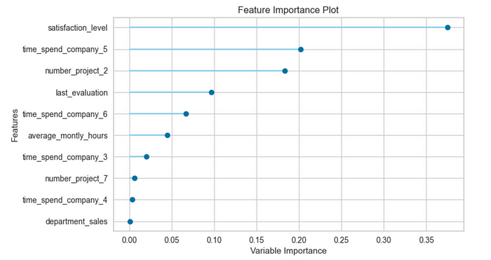
Pycaret has a selection of built-in plots to interpret the results of the model which can be accessed using the plot_model() function.
Below we inspect feature importances using this function.https://towardsdatascience.com/media/6eab5425185437e03116c0164afd2b6b
Let’s also visualise the confusion matrix.https://towardsdatascience.com/media/5399f3c6430eea1ecbf7473890f877af

Deploy the model
Pycaret has additional functionality to deploy models to the cloud using AWS.
To deploy the model on AWS you must first create an account on aws.amazon.com. Once created you need to generate an access key so that you can allow the Pycaret function to write to your account. To do this follow the following steps.
- Login to your AWS account.
- Hover over your username in the top right corner.
- Select security credentials from the list that appears.

4. From here expand the Access keys section and click on ‘Create new access key’.

5. At this stage you need to download the credentials file when prompted. You will need the credentials contained file in this later.
6. To allow Pycaret to interact with your AWS account you also need to install and configure the AWS CLI. To do this first run the following.
curl "https://awscli.amazonaws.com/AWSCLIV2.pkg" -o "AWSCLIV2.pkg"
Then run this:
sudo installer -pkg ./AWSCLIV2.pkg -target /
Now type aws --version to confirm everything has been installed correctly. You should see something like this.

Now that this is installed we can configure the AWS CLI with your account details. To do this run the command shown below. It will ask you to input the following pieces of information.
AWS Access Key ID: this can be found in the credentials file we downloaded earlier.
AWS Secret Acess Key: also found in the credentials file.
Default region name: this can be found on the AWS console.
Default output format: this should be left blank.
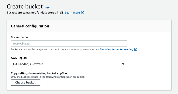
Next, we create an S3 bucket to store the deployed model. From the AWS console select S3 and then create a bucket with your chosen name.
Now we are ready to use Pycaret to deploy our chosen model.https://towardsdatascience.com/media/87b9c733f312a0442ff6494eeb1ad3ae
If the model has deployed you will see the following message.

Generate predictions
To use the model we generate predictions on the validation data we reserved earlier.
The code shown below loads the model from S3 and generates predictions on the validation data with the labels removed.https://towardsdatascience.com/media/5becc725087b039c6403cad17bfb6d5f
Let’s view the first 5 predictions by running predictions[:5].

Monitoring
An important aspect of the production machine learning workflow is tracking and monitoring the experiments that are performed. Pycaret has integration with MLflow an open-source platform for managing the end to end machine learning lifecycle.
To use MLflow via Pycaret we need to import MLflow (this should already have been installed along with Pycaret) and set the tracking URI. We then add a couple of extra parameters as shown below when calling the setup function.https://towardsdatascience.com/media/99b922bca8501163398955b720c39d61
Now if we copy the tracking URI into a browser you should see the mlflow UI and the experiments it has tracked.

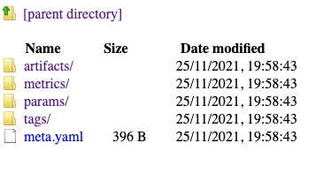
We can click through to view the metrics, artifacts and params for each experiment performed.
This is a simple tutorial to learn the basic steps involved in an end to end machine learning project. In the real world most machine learning problems, data and deployment solutions require much more complex treatment. However, for the purposes of this tutorial I have used a simple dataset and python library to get you started with learning about the end to end machine learning lifecycle.
Pycaret is an example of a low-code machine learning library. There are a number of tools being developed that seek to simplify machine learning development in different ways. To learn more about these low effort machine learning libraries see my earlier article.
Rebecca Vickery Data Scientist | Writer, Speaker, Founder DatAcademy |


